Expression Templates Library (ETL) 1.1

ETL Logo

It took me longer than I thought, but I'm glad to announce the release of the version 1.1 of my Expression Templates Library (ETL) project. This is a major new release with many improvements and new features. It's been almost one month since the last, and first, release (1.0) was released. I should have done some minor releases in the mean time, but at least now the library is in a good shape for major version.

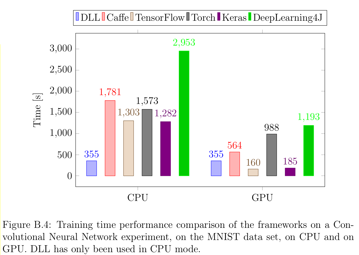
It may be interesting to note that my machine learning framework (DLL), based on the ETL library, has shown to be faster than all the tested popular frameworks (Tensorflow, Keras, Caffee, Torch, DeepLearning4J) for training various neural networks on CPU. I'll post more details on another post on the coming weeks, but that shows that special attention to performance has been done in this library and that it is well adapted to machine learning.

For those of you that don't follow my blog, ETL is a library providing Expression Templates for computations on matrix and vector. For instance, if you have three matrices A, B and C you could write C++ code like this:

C = (2.0 * (A + B)) / sum(A)

Or given vectors b, v, h and a matrix W, you could write code like this:

h = sigmoid(b + v * W)

The goal of such library is two-fold. First, this makes the expression more readable and as close to math as possible. And then, it allows the library to compute the expressions as fast as possible. In the first case, the framework will compute the sum using a vectorized algorithm and then compute the overall expression using yet again vectorized code. The expression can also be computed in parallel if the matrices are big enough. In the second case, the vector-matrix multiplication will be computed first using either hand-code optimized vectorized or a BLAS routine (depending on configuration options). Then, all the expression will be executed using vectorized code.

Features

Many new features have been integrated into the library.

The support for machine learning operations has been improved. There are now specific helpers for machine learning in the etl::ml namespace which have names that are standard to machine learning. A real transposed convolution has been implemented with support for padding and stride. Batched outer product and batched bias averaging are also now supported. The activation function support has also been improved and the derivatives have been reviewed. The pooling operators have also been improved with stride and padding support. Unrelated to machine learning, 2D and 3D pooling can also be done in higher dimensional matrix now.

New functions are also available for matrices and vectors. The support for square root has been improved with cubic root and inverse root. Support has also been added for floor and ceil. Moreover, comparison operators are now available as well as global functions such as approx_equals.

New reductions have also been added with support for absolute sum and mean (asum/asum) and for min_index and max_index, which returns the index of the minimum element, respectively the maximum. Finally, argmax can now be used to get the max index in each sub dimensions of a matrix. argmax on a vector is equivalent to max_index.

Support for shuffling has also been added. By default, shuffling a vector means shuffling all elements and shuffling a matrix means shuffling by shuffling the sub matrices (only the first dimension is shuffled), but shuffling a matrix as a vector is also possible. Shuffle of two vectors or two matrices in parallel, is also possible. In that case, the same permutation is applied to both containers. As a side note, all operations using random generation are also available with an addition parameter for the random generator, which can help to improve reproducibility or simply tune the random generator.

I've also included support for adapters matrices. There are adapters for hermitian matrices, symmetric matrices and lower and upper triangular matrices. For now, the framework does not take advantage of this information, this will be done later, but the framework guarantee the different constrain on the content.

There are also a few new more minor features. Maybe not so minor, matrices can now be sliced into sub matrices. With that a matrix can be divided into several sub matrices and modifying the sub matrices will modify the source matrix. The sub matrices are available in 2D, 3D and 4D for now. There are also some other ways of slicing matrix and vectors. It is possible to obtain a slice of its memory or obtain a slice of its first dimension. Another new feature is that it is now possible compute the cross product of vectors now. Matrices can be decomposed into their Q/R decomposition rather than only their PALU decomposition. Special support has been integrated for matrix and vectors of booleans. In that case, they support logical operators such as and, not and or.

Performance

I've always considered the performance of this library to be a feature itself. I consider the library to be quite fast, especially its convolution support, even though there is still room for improvement. Therefore, many improvements have been made to the performance of the library since the last release. As said before, this library was used in a machine learning framework which then proved faster than most popular neural network frameworks on CPU. I'll present here the most important new improvements to performance, in no real particular order, every bit being important in my opinion.

First, several operations have been optimized to be faster.

Multiplication of matrices or matrices and vectors are now much faster if one of the matrix is transposed. Instead of performing the slow transposition, different kernels are used in order to maximize performance without doing any transposition, although sometimes transposition is performed when it is faster. This leads to very significant improvements, up to 10 times faster in the best case. This is performed for vectorized kernels and also for BLAS and CUBLAS calls. These new kernels are also directly used when matrices of different storage order are used. For instance, multiplying a column major matrix with a row major matrix and storing the result in a column major matrix is now much more efficient than before. Moreover, the performance of the transpose operation itself is also much faster than before.

A lot of machine learning operations have also been highly optimized. All the pooling and upsample operators are now parallelized and the most used kernel (2x2 pooling) is now more optimized. 4D convolution kernels (for machine learning) have been greatly improved. There are now very specialized vectorized kernels for classic kernel configurations (for instance 3x3 or 5x5) and the selection of implementations is now smarter than before. The support of padding is now much better than before for small amount of padding. Moreover, for small kernels the full convolution can now be evaluated using the valid convolution kernels directly with some padding, for much faster overall performance. The exponential operation is now vectorized which allows operations such as sigmoid or softmax to be much faster.

Matrices and vector are automatically using aligned memory. This means that vectorized code can use aligned operations, which may be slightly faster. Moreover, matrices and vectors are now padded to a multiple of the vector size. This allows to remove the final non-vectorized remainder loop from the vectorized code. This is only done for the end of matrices, when they are accessed in flat way. Contrary to some frameworks, inner dimensions of the matrix are not padded. Finally, accesses to 3D and 4D matrices is now much faster than before.

Then, the parallelization feature of ETL has been completely reworked. Before, there was a thread pool for each algorithm that was parallelized. Now, there is a global thread engine with one thread pool. Since parallelization is not nested in ETL, this improves performance slightly by greatly diminishing the number of threads that are created throughout an application. Another big difference in parallel dispatching is that now it can detect good split based on alignment so that each split are aligned. This then allows the vectorization process to use aligned stores and loads instead of unaligned ones which may be faster on some processors.

Vectorization has also been greatly improved in ETL. Integer operations are now automatically vectorized on processors that support this. Before, only floating points operations were vectorized. The automatic vectorizer now is able to use non-temporal stores for very large operations. A non-temporal store bypasses the cache, thus gaining some time. Since very large matrices do not fit in cache anyway and the cache would end up being overwritten anyway, this is a net gain. Moreover, the alignment detection in the automatic vectorizer has also been improved. Support for Fused-Multiply-Add (FMA) operations has also been integrated in the algorithms that can make use of it (multiplications and convolutions). The matrix-matrix multiplications and vector-matrix multiplications now have highly optimized vectorized kernels. They also have versions for column-major matrices now. I plan to reintegrate a version of the GEMM based on BLIS in the future but with more optimizations and support for all precisions and integers, For my version is still slower than the simple vectorized version. The sum and the dot product operations now also have specialized vectorized implementations. The min and max operations are now automatically-vectorized. Several others algorithms have also their own vectorized implementations.

Last, but not least, the GPU support has also been almost completely reworked. Now, several operations can be chained without any copies between GPU and CPU. Several new operations have also been added with support to GPU (convolutions, pooling, sigmoid, ReLU, ...). Moreover, to complement operations that are not available in any of the supported NVIDIA libraries, I've created a simple library that can be used to add a few more GPU operations. Nevertheless a lot of operations are still missing and only algorithms are available not expressions (such as c = a + b * 1.0) that are entirely computed on CPU. I have plans to improve that further, probably for version 1.2. The different contexts necessary for NVIDIA library can now be cached (using an option from ETL), leading to much faster code. Only the main handle can be cached so far, I plan to try to cache all the descriptors, but I don't know yet when that will be ready. Finally, an option is also available to reuse GPU memory instead of directly releasing it to CUDA. This is using a custom memory pool and can save some time. Since this needs to be cleaned (by a call to etl::exit() or using ETL_PROLOGUE), this is only activated on demand.

Other changes

There also have been a lot of refactorings in the code of the library. A lot of expressions now have less overhead and are specialized for performance. Moreover, temporary expressions have been totally reworked to be more simple and maintainable and easier to optimize in the future. It's also probably easier to add new expressions to the framework now, although that could be even more simple. There are also less duplicated code now in the different expressions. Especially, now there are now more SSE and AVX variants in the code. All the optimized algorithms are now using the vectorization system of the library.

I also tried my best to reduce the compilation time, based on the unit tests. This is still not great but better than before. For user code, the next version should be much faster to compile since I plan to disable forced selection of implementations by default and only enable it on demand.

Finally, there also was quite a few bug fixes. Most of them have been found by the use of the library in the Deep Learning Library (DLL) project. Some were very small edge cases. For instance, the transposition algorithm was not working on GPU on rectangular column major matrices. There also was a slight bug in the Q/R decomposition and in the pooling of 4D matrices.

What's next ?

Next time, I may do some minor release, but I don't yet have a complete plan. For the next major release (1.2 probably), here is what is planned:

  • Review the system for selection of algorithms to reduce compilation time

  • Review the GPU system to allow more complete support for standard operators

  • Switch to C++17: there are many improvements that could be done to the code with C++17 features

  • Add support for convolution on mixed types (float/double)

  • More tests for sparse matrix

  • More algorithms support for sparse matrix

  • Reduce the compilation time of the library in general

  • Reduce the compilation and execution time of the unit tests

These are pretty big changes, especially the first two, so maybe it'll be split into several releases. It will really depend on the time I have. As for C++17, I really want to try it and I have a lot of points that could profit from the switch, but that will means setting GCC 7.1 and Clang 3.9 as minimum requirement, which may not be reasonable for every user.

Download ETL

You can download ETL on Github. If you only interested in the 1.1 version, you can look at the Releases pages or clone the tag 1.1. There are several branches:

  • master Is the eternal development branch, may not always be stable

  • stable Is a branch always pointing to the last tag, no development here

For the future release, there always will tags pointing to the corresponding commits. I'm not following the git flow way, I'd rather try to have a more linear history with one eternal development branch, rather than an useless develop branch or a load of other branches for releases.

The documentation is a bit sparse. There are a few examples and the Wiki, but there still is work to be done. If you have questions on how to use or configure the library, please don't hesitate.

Don't hesitate to comment this post if you have any comment on this library or any question. You can also open an Issue on Github if you have a problem using this library or propose a Pull Request if you have any contribution you'd like to make to the library.

Hope this may be useful to some of you :)

Update on Deep Learning Library (DLL): Dropout, Batch Normalization, Adaptive Learning Rates, ...

It's been a while since I've posted something on this, especially since I had one month vacation. This year I've been able to integrate a great number of changes into my Deep Learning Library (DLL) project. It has seen a lot of refactorings and a lot of new features making it look like a real neural network library now. In this post, I'll try to outline the last new features and changes of the library.

For those that don't know, DLL is a library for neural network training, written in C++ and for C++. You can train Fully-Connected Neural Networks and Convolutional Neural Networks. The focus of the framework is on speed and easy use in C++.

As for my ETL project and again thanks to my thesis supervisor, the project now has a logo:

DLL Logo

Adaptive Learning Rates

Before, the framework only supported simple SGD and Momentum updates for the different parameters of the network. Moreover, it was not very well extendable. Therefore, I reviewed the system to be able to configure an optimizer for each network to train. Once that was done, the first thing I did was to add support for Nesterov Accelerated Gradients (NAG) as a third optimizer. After this, I realized it was then easy to integrate support for more advanced optimizers including support for adaptive learning rates. This means that the learning rate will be adapted for each parameter depending on what the network is learning. Some of the optimizers even don't need any learning rate. So far, I've implemented support for the following optimizers: Adagrad, RMSProp, Adam (with and without bias correction), Adamax (Adam with infinite norm), Nadam (Adam with Nesterov momentum) and Adadelta (no more learning rate). The user can now choose the optimizer of its choice, for instance NADAM, as a parameter of the network:

// Use a Nadam optimizer
dll::updater<dll::updater_type::NADAM>

Another improvement in the same domain is that the learning rate can also be decayed over time automatically by the optimizer.

If you want more information on the different optimizers, you can have a look at this very good article: An overview of gradient descent optimization algorithms from Sebastian Ruder.

Better loss support

Before, DLL was automatically using Categorical Cross Entropy Loss, but it was not possible to change it and it was not even possible to see the loss over time. Now, the current value of the loss is displayed after each epoch of training and the loss used for training is now configurable. So far, only three different losses are supported, but it it not difficult to add new loss to the system. The three losses supported are: Categorical Cross Entropy Loss, Binary Cross Entropy Loss and Mean Squared Error Loss.

Again, each network can specify the loss to use:

// Use a Binary Cross Entropy Loss
dll::loss<dll::loss_function::BINARY_CROSS_ENTROPY>

Dropout

Dropout is a relatively new technique for neural network training. This is especially made to reduce overfitting since a large number of sub networks will be trained and it should prevent co-adaptation between different neurons. This technique is relatively simple. Indeed, it simply randomly sets to zero some of the input neurons of layers. At each batch, a new mask will be used and this should lead to a large number of sub networks being trained.

Here is example of a MLP with Dropout (p=0.5):

using network_t = dll::dyn_dbn_desc<
    dll::dbn_layers<
        dll::dense_desc<28 * 28, 500>::layer_t,
        dll::dropout_layer_desc<50>::layer_t,
        dll::dense_desc<500, 250>::layer_t,
        dll::dropout_layer_desc<50>::layer_t,
        dll::dense_desc<250, 10, dll::activation<dll::function::SOFTMAX>>::layer_t>
    , dll::updater<dll::updater_type::MOMENTUM>     // Momentum
    , dll::batch_size<100>                          // The mini-batch size
    , dll::shuffle                                  // Shuffle before each epoch
>::dbn_t;

Batch Normalization

Batch Normalization is another new technique for training neural networks. This technique will ensure that each of the layer will receive inputs that look kind of similar. This is a very large advantage since then you reduce the different in impact of hyper parameters on different layers. Google reported much faster training with this technique by getting rid of Dropout and by increasing the learning rate of training.

Here is an example of using Batch Normalization in a CNN:

using network_t = dll::dyn_dbn_desc<
    dll::dbn_layers<
        dll::conv_desc<1, 28, 28, 8, 5, 5>::layer_t,
        dll::batch_normalization_layer_4d_desc<8, 24, 24>::layer_t,
        dll::mp_layer_2d_desc<8, 24, 24, 2, 2>::layer_t,
        dll::conv_desc<8, 12, 12, 8, 5, 5>::layer_t,
        dll::batch_normalization_layer_4d_desc<8, 8, 8>::layer_t,
        dll::mp_layer_2d_desc<8, 8, 8, 2, 2>::layer_t,
        dll::dense_desc<8 * 4 * 4, 150>::layer_t,
        dll::batch_normalization_layer_2d_desc<150>::layer_t,
        dll::dense_desc<150, 10, dll::activation<dll::function::SOFTMAX>>::layer_t>
    , dll::updater<dll::updater_type::ADADELTA>     // Adadelta
    , dll::batch_size<100>                          // The mini-batch size
    , dll::shuffle                                  // Shuffle the dataset before each epoch
>::dbn_t;

You may notice that the layer is set as 4D so should only be used after convolutional layer (or after the input). If you want to use it after fully-connected layers, you can use the 2D version that works the same way.

Better dataset support

At the beginning, I designed DLL so that the user could directly pass data for training in the form of STL Containers such as the std::vector. This is good in some cases, but in some cases, the user does not know how to read the data , or does not want to be bothered with it. Therefore, several data sets reader are now available. Moreover, the entire system has been reworked to use generators for data. A generator is simply a concept that has some data to produce. The advantage of this new system is data augmentation is now supported every where and much more efficiently than before. It is now possible to perform random cropping and mirroring of images for instance. Moreover, the data augmentation can be done in a secondary thread so as to be sure that there is always enough data available for the training.

The library now has a powerful dataset reader for both MNIST and CIFAR-10 and the reader for ImageNet is almost ready. The project has already been used and tested with these three datasets now. Moreover, the support for directly passing STL containers has been maintained. In this case, a generator is simply created around the data provided in the container and the generator is then passed to the system for training.

Here for instance is how to read MNIST data and scale (divide) all pixel values by 255:

// Load the dataset
auto dataset = dll::make_mnist_dataset(0, dll::batch_size<100>{}, dll::scale_pre<255>{});
dataset.display();

// Train the network
net->fine_tune(dataset.train(), 25);

// Test the network
net->evaluate(dataset.test());

Much faster performance

I've spent quite a lot of time improving the performance of the framework. I've focused on every part of training in order to make training of neural networks as fast as possible. I've also made a comparison of the framework against several popular machine learning framework (Caffe, TensorFlow, Keras, Torch and DeepLearning4J). For instance, here are the results on a small CNN experiment on MNIST with all the different frameworks in CPU mode and in GPU mode:

DLL Comparison Against other frameworks

As you can see, DLL is by far the fastest framework on CPU. On GPU, there is still some work to be done, but this is already ongoing (although a lot of work remains). This is confirmed on each of the four experiments performed on MNIST, CIFAR-10 and ImageNet, although the margin is smaller for larger networks (still about 40% faster than TensorFlow and Keras which are the fastest framework after DLL on CPU on my tests).

Overall, DLL is between 2 and 4 times faster than before and is always the fastest framework for neural network training when training is performed on CPU.

I proposed a talk about these optimizations and performance for Meeting C++ this year, but it has unfortunately not been accepted. We also have submitted a publication about the framework to a conference later this year.

Examples

The project now has a few examples (available here), well-designed and I try to update them with the latest updates of the framework.

For instance, here is the CNN example for MNIST (without includes):

int main(int /*argc*/, char* /*argv*/ []) {
    // Load the dataset
    auto dataset = dll::make_mnist_dataset(0, dll::batch_size<100>{}, dll::scale_pre<255>{});

    // Build the network

    using network_t = dll::dyn_dbn_desc<
        dll::dbn_layers<
            dll::conv_desc<1, 28, 28, 8, 5, 5>::layer_t,
            dll::mp_layer_2d_desc<8, 24, 24, 2, 2>::layer_t,
            dll::conv_desc<8, 12, 12, 8, 5, 5>::layer_t,
            dll::mp_layer_2d_desc<8, 8, 8, 2, 2>::layer_t,
            dll::dense_desc<8 * 4 * 4, 150>::layer_t,
            dll::dense_desc<150, 10, dll::activation<dll::function::SOFTMAX>>::layer_t>
        , dll::updater<dll::updater_type::MOMENTUM>     // Momentum
        , dll::batch_size<100>                          // The mini-batch size
        , dll::shuffle                                  // Shuffle the dataset before each epoch
    >::dbn_t;

    auto net = std::make_unique<network_t>();

    net->learning_rate = 0.1;

    // Display the network and dataset
    net->display();
    dataset.display();

    // Train the network
    net->fine_tune(dataset.train(), 25);

    // Test the network on test set
    net->evaluate(dataset.test());

    return 0;
}

Reproducible results

And last, but maybe not least, I've finally united all the random number generation code. This means that DLL can now set a global seed and that two training of the same network and data with the same seed will now produce exactly the same result.

The usage is extremely simple:

dll::set_seed(42);

Conclusion

After all these changes, I truly feel that the library is now in a much better state and could be useful in several projects. I hope that this will be useful to some more people. Moreover, as you can see by the performance results, the framework is now extremely efficient at training neural networks on CPU.

If you want more information, you can consult the dll Github Repository. You can also add a comment to this post. If you find any problem on the project or have specific question or request, don't hesitate to open an issue on Github.

Jenkins Tip: Send notifications on fixed builds in declarative pipeline

In my previous post, I presented a few news about Jenkins and about the fact that I switched to declarative pipelines and Github Organization support for my projects.

The main issue I had with this system is that I lost the ability to get notifications on build that recover. Normally, I would get an email indicating that build X was back to normal, but I haven't found a way to solve that for declarative pipeline.

By following a few posts on StackOverflow, I now have the solution and it is the same problem that was already present in scripted pipelines. Namely, the status of the current build is not set early enough for the notification. Basically, you have to set the notification yourself. Here is what a declarative pipeline looks like:

pipeline {
    agent any

    stages {

        // Normal Stages

        stage ('success'){
            steps {
                script {
                    currentBuild.result = 'SUCCESS'
                }
            }
        }
    }

    post {
        failure {
            script {
                currentBuild.result = 'FAILURE'
            }
        }

        always {
            step([$class: 'Mailer',
                notifyEveryUnstableBuild: true,
                recipients: "[email protected]",
                sendToIndividuals: true])
        }
    }
}

There are two important things here. First, a new stage (success) is added that simply set the result of the current build to SUCCESS once it is done. It must be the last stage on the pipeline. This could also be added as the last step of the last stage instead of adding a new stage, but I think it's clearer like this. The second thing is the failure block in which the result of the current build is set to FAILURE. With these two things, the Mailer plugin now sends notification when a build has been fixed.

I hope that will help some of you. I personally think that it should be much easier than that. All this boilerplate is polluting the pipeline that should be kept more maintainable, but for now it seems, it's the nicest way to achieve that, short of handling all conditions in the post block and sending mail directly there, but that would result in even more boilerplate code.

Jenkins Declarative Pipeline and Awesome Github Integration

This post is about some news about Jenkins and how I've updated my Jenkins usage. This may be a bit of an enthusiastic post ;)

At the beginning of Jenkins, the best way to define the commands to be executed for your builds was simply to write the commands in the Jenkins interface. This worked quite well. Later on, Jenkins introduced the notion of Pipeline. Instead of a single set of commands to be executed, the build was defined in multi-stages pipeline of commands. This is defined as a Groovy script. One big advantage of this is that all the code for creating the build is inside the repository. This has the advantage that each build is reproducible. This enabled to define complex pipelines of commands for your builds. Moreover, this also allows to have a clean view of which steps are failing and which steps are taking how much of the time of the build. For instance, here it's a view of the pipeline steps for my DLL project:

Jenkins stage view for DLL pipeline.

I think that's pretty cool :)

They recently added a new feature, the declarative pipelines. Instead of scripting the Pipeline in Groovy, the new system uses its own syntax, completely declarative, to put blocks together and add ways of doing actions at specific points and setting environment and so on. I think the new syntax is much nicer than the Groovy scripted Pipeline way, so I started converting my scripts. I'll give an example in a few paragraphs. But first, I'd like to talk about Github integration. Before, every time I created a new project, I add to add it to Jenkins by creating a new project, updating the link to the Github project and a few things in order to add it. This is not so bad but what if you want to build on several branches and keep track of the status of the branches and maybe of the Pull Requests as well. All of this is now very simple. You can now declare the Github organizations (and users) you are of building projects from and the projects inside the organization will be automatically detected as long as they have a Jenkinsfile inside. That means that you'll never have to create a project yourself or handle branches. Indeed, all the created projects can now handle multiples. For instance, here is the status of the two current branches of my dll project:

Jenkins branches for DLL Github project

It's maybe not the best example since one branch is failing and the other is unstable, but you can see that you can track the builds for each branch in a nice way.

A very good feature of this integration is that Jenkins will now automatically marks commits on your Github with the status of your builds at no cost! For instance, here is the status on my ETL project after I configured on Jenkins and made the first builds:

Jenkins marking commits in Github

Pretty cool I think :)

Another nice thing in Jenkins is the Blue Ocean interface. This is an alternative interface, especially well-suited for multi-branch projects and pipelines. It looks much more modern and I think it's quite good. Here are a few views of it:

The Activity view for the last events of the project:

Jenkins Blue Ocean Activity view for DLL project

The Branches view for the status of each branch:

Jenkins Blue Ocean Branches view for DLL project

The view of the status of a build:

Jenkins Blue Ocean view of a build for DLL project

The status of the tests for a given build:

Jenkins Blue Ocean view of a build tests for DLL project

It's likely that it won't appeal to everyone, but I think it's pretty nice.

If we get back to the declarative Pipeline, here is the declarative pipeline for my Expression Templates Library (ETL) project:

pipeline {
    agent any

    environment {
       CXX = "g++-4.9.4"
       LD = "g++-4.9.4"
       ETL_MKL = 'true'
    }

    stages {
        stage ('git'){
            steps {
                checkout([
                    $class: 'GitSCM',
                    branches: scm.branches,
                    doGenerateSubmoduleConfigurations: false,
                    extensions: scm.extensions + [[$class: 'SubmoduleOption', disableSubmodules: false, recursiveSubmodules: true, reference: '', trackingSubmodules: false]],
                    submoduleCfg: [],
                    userRemoteConfigs: scm.userRemoteConfigs])
            }
        }

        stage ('pre-analysis') {
            steps {
                sh 'cppcheck --xml-version=2 -j3 --enable=all --std=c++11 `git ls-files "*.hpp" "*.cpp"` 2> cppcheck_report.xml'
                sh 'sloccount --duplicates --wide --details include/etl test workbench > sloccount.sc'
                sh 'cccc include/etl/*.hpp test/*.cpp workbench/*.cpp || true'
            }
        }

        stage ('build'){
            steps {
                sh 'make clean'
                sh 'make -j6 release'
            }
        }

        stage ('test'){
            steps {
                sh 'ETL_THREADS=-j6 ETL_GPP=g++-4.9.4 LD_LIBRARY_PATH=\"${LD_LIBRARY_PATH}:/opt/intel/mkl/lib/intel64:/opt/intel/lib/intel64\" ./scripts/test_runner.sh'
                archive 'catch_report.xml'
                junit 'catch_report.xml'
            }
        }

        stage ('sonar-master'){
            when {
                branch 'master'
            }
            steps {
                sh "/opt/sonar-runner/bin/sonar-runner"
            }
        }

        stage ('sonar-branch'){
            when {
                not {
                    branch 'master'
                }
            }
            steps {
                sh "/opt/sonar-runner/bin/sonar-runner -Dsonar.branch=${env.BRANCH_NAME}"
            }
        }

        stage ('bench'){
            steps {
                build job: 'etl - benchmark', wait: false
            }
        }
    }

    post {
        always {
            step([$class: 'Mailer',
                notifyEveryUnstableBuild: true,
                recipients: "[email protected]",
                sendToIndividuals: true])
        }
    }
}

There is nothing really fancy about, it's probably average. Moreover, since I'm not an expert on pipelines and I've just discovered declarative pipelines, it may not be optimal, but it works. As you'll see there are some problems I haven't been able to fix.

The first part declares the environment variables for the build. Then, the multiple build stages are listed. The first stage checkout the code from the SCM. This ugly piece of code is here to allow to checkout the submodules. It is the only solution I have found so far. It's very ugly but it works. The second steps is simply some basic static analysis. The next step is the classical build step. Then, the tests are run. In that case, I'm using a script because the tests are compiled with several different sets of options and it was much easier to put that in a script that in the Pipeline. Moreover, that also means I can run them standalone. The variables in the line to run the script is another problem I haven't been able to fix so far. If I declare these variables in an environment block, they are not passed to the script for some reason, so I had to use this ugly line. The next two blocks are for Sonar analysis. If you start with Sonar, you can simply the second block that passed the branch information to Sonar. Unfortunately, Sonar is very limited in terms of Git branches. Each branch is considered as another totally different project. That means the false positives defined in the master branch will not be used in the second branch. Therefore, I kept a clean master and several different projects for the other branches. Once Sonar improves this branch handling stuff, if they ever do, I'll be able to get rid of one of these conditional stages. The last stage is simple running the benchmark job. Finally, the post block is using the Mailer plugin to send failed builds information. Again, there is a problem here since this does not send "Back to normal" information as it used to do before. I've asked this question on StackOverflow, but haven't received an answer so far. I'll post a better solution on this blog once I have one. If any of you have some solutions to these problems, don't hesitate to post in the comments below or to contact me on Github.

Here it is. I really think Jenkins is getting even greater now with all this cool stuff and I advice you to try it out!

C++ Containers Benchmark: vector/list/deque and plf::colony

Already more than three years ago, I've written a benchmark of some of the STL containers, namely the vector, the list and the deque. Since this article was very popular, I decided to improve the benchmarks and collect again all the results. There are now more benchmarks and some problems have been fixed in the benchmark code. Moreover, I have also added a new container, the plf::colony. Therefore, there are four containers tested:

  • The std::vector: This is a dynamically-resized array of elements. All the elements are contiguous in memory. If an element is inserted or removed it at a position other than the end, the following elements will be moved to fill the gap or to open a gap. Elements can be accessed at random position in constant time. The array is resized so that it can several more elements, not resized at each insert operation. This means that insertion at the end of the container is done in amortized constant time.

  • The std::deque: The deque is a container that offer constant time insertion both at the front and at the back of the collection. In current c++ libraries, it is implementation as a collection of dynamically allocated fixed-size array. Not all elements are contiguous, but depending on the size of the data type, this still has good data locality. Access to a random element is also done in constant time, but with more overhead than the vector. For insertions and removal at random positions, the elements are shifted either to the front or to the back meaning that it is generally faster than the vector, by twice in average.

  • The std::list: This is a doubly-linked list. It supports constant time insertions at any position of the collection. However, it does not support constant time random access. The elements are obviously not contiguous, since they are all allocated in nodes. For small elements, this collection has a very big memory overhead.

  • The plf::colony: This container is a non-standard container which is unordered, it means that the insertion order will not necessarily be preserved. It provides strong iterators guarantee, pointers to non-erased element are not invalidated by insertion or erasure. It is especially tailored for high-insertion/erasure workloads. Moreover, it is also specially optimized for non-scalar types, namely structs and classes with relatively large data size (greater than 128 bits on the official documentation). Its implementation is more complicated than the other containers. It is also implemented as a list of memory blocks, but they are of increasingly large sizes. When elements are erased, there position is not removed, but marked as erased so that it can be reused for fast insertion later on. This container uses the same conventions as the standard containers and was proposed for inclusion to the standard library, which is the main reason why it's included in this benchmark. If you want more information, you can consult the official website.

In the text and results, the namespaces will be omitted. Note that I have only included sequence containers in my test. These are the most common containers in practices and these also the containers I'm the most familiar with. I could have included multiset in this benchmark, but the interface and purpose being different, I didn't want the benchmark to be confusing.

All the examples are compiled with g++-4.9.4 (-std=c++11 -march=native -O2) and run on a Gentoo Linux machine with an Intel Core i7-4770 at 3.4GHz.

For each graph, the vertical axis represent the amount of time necessary to perform the operations, so the lower values are the better. The horizontal axis is always the number of elements of the collection. For some graph, the logarithmic scale could be clearer, a button is available after each graph to change the vertical scale to a logarithmic scale.

The tests are done with several different data types. The trivial data types are varying in size, they hold an array of longs and the size of the array varies to change the size of the data type. The non-trivial data type is composed of a string (just long enough to avoid SSO (Small String Optimization) (even though I'm using GCC)). The non-trivial data types comes in a second version with noexcept move operations. Not all results are presented for each data types if there are not significant differences between in order to keep this article relatively short (it's already probably too long :P).

Read more…

Speed up TensorFlow inference by compiling it from source

The most simple way to install TensorFlow is to work in a virtual Python environment and simply to use either the TensorFlow official packages in pip or use one of the official wheels for distributions. There is one big problem with that technique and it's the fact that the binaries are precompiled so that they fit as many hardware configuration as possible. This is normal from Google since generating precompiled binaries for all the possible combinations of processor capabilities would be a nightmare. This is not a problem for GPU since the CUDA Libraries will take care of the difference from one graphics card to another. But it is a problem with CPU performance. Indeed, different processors have different capabilities. For instance, the vectorization capabilities are different from processor to processor (SSE, AVX, AVX2, AVX-512F, FMA, ...). All those options can make a significant difference in the performance of the programs. Although most of the machine learning training occurs on GPU most of the time, the inference is mostly done on the CPU. Therefore, it probably remains important to be as fast as possible on CPU.

So if you care about performance on CPU, you should install TensorFlow from sources directly yourself. This will allow compilation of the TensorFlow sources with -march=native which will enable all the hardware capabilities of machine on which you are compiling the library.

Depending on your problem, this may give you some nice speedup. In my case, on a very small Recurrent Neural Network, it made inference about 20% faster. On a larger problem and depending on your processor, you may gain much more than that. If you are training on CPU, this may make a very large difference in total time.

Installing TensorFlow is sometimes a bit cumbersome. You'll likely have to compile Bazel from sources as well and depending on your processor, it may take a long time to finish. Nevertheless, I have successfully compiled TensorFlow from sources on several machines now without too many problems. Just pay close attention to the options you are setting while configuring TensorFlow, for instance CUDA configuration if you want GPU support.

I hope this little trick will help you gain some time :)

Here is the link to compile TensorFlow from source.

Update on Expression Templates Library (ETL)

It's been a while since I've released the version 1.0 of ETL. There is some work to do before I release the next version, but I wanted to give you a quick update on what has been going on for ETL in the last months. There has been a lot of changes in the library and the next version will be a major update when I'm done with some refactorings and improvements.

Thanks to my thesis supervisor, the project now has a logo:

ETL Logo

There are quite a few new features, although probably nothing really major. The support for square root has been improved with cubic root and inverse root. Vectors can now be transformed using floor and ceil. Cross product of vector has been implemented as well. Batched outer product and batched bias averaging (for machine learning) are now supported. Reductions have also been improved with absolute sum and mean (asum/asum) support and min_index and max_index. argmax can now be used to get the max index in each sub dimensions. Matrix can now be decomposed into their Q/R decomposition rather than only their PALU decomposition. The matrices can now be sliced by getting only a sub part of the matrix. The pooling operators have also been improved with stride and padding support. Matrices and vectors can also be shuffled. Moreover, a few adapters are now available for hermitian matrices, symmetric matrices and lower and upper matrices. So far the support for these adapters is not huge, but they are guaranteed to validate their constraints.

Several operations have been optimized for speed. All the pooling and upsample operators are now parallelized and the most used kernel (2x2 pooling) is now more optimized. 4D convolution kernels (for machine learning) have been greatly improved. There are now very specialized vectorized kernels for classic kernel configurations (for instance 3x3 or 5x5) and the selection of implementations is now smarter than before. The support of padding now much better than before for small amount of padding. Moreover, for small kernels the full convolution can now be evaluated using the valid convolution kernels directly with some padding, for much faster overall performance. Matrix-matrix multiplication with transposed matrices is now much faster when using BLAS kernels. Indeed, the transposition is not performed but handled inside the kernels. Moreover, the performance of the transposition itself is also much faster. Finally, accesses to 3D and 4D matrices is now much faster than before.

The parallelization feature of ETL has been completely reworked. Before, there was a thread pool for each algorithm that was parallelized. Now, there is a global thread engine with one thread pool. Since parallelization is not nested in ETL, this improves performance slightly by greatly diminishing the number of threads that are created throughout an application.

Vectorization has also been greatly improved in ETL. Integer operations are now automatically vectorized on processors that support this. The automatic vectorizer now is able to use non-temporal stores for very large operations. A non-temporal store bypasses the cache, thus gaining some time. Since very large matrices do not fit in cache, this is a net gain. Moreover, the alignment detection in the automatic vectorizer has also been improved. Support for Fused-Multiply-Add (FMA) operations has also been integrated in the algorithms that can make use of it. The matrix-matrix multiplications and vector-matrix multiplications now have optimized vectorized kernels. They also have versions for column-major matrices now. The old egblas version of the gemm, based on BLIS kernels, has been removed since it was only supporting double-precision and was not faster than the new vectorized algorithm. I plan to reintegrate a version of the GEMM based on BLIS in the future but with more optimizations and support for all precisions and integers. The sum and the dot product now also have specialized vectorized implementations. The min and max operations are now automatically-vectorized.

The GPU has also been almost completely reworked. Now, operations can be chained without any copies between GPU and CPU. Several new operations have also been added with support to GPU. Moreover, to complement operations that are not available in any of the supported NVIDIA libraries, I've created a simple library that can be used to add a few more GPU operations. Nevertheless a lot of operations are still missing and only algorithms are available not expressions (such as c = a + b * 1.0) that are entirely computed on CPU. I have plans to improve that further, but probably not before the version 1.2.

There also have been a lot of refactorings in the code of the library. A lot of expressions now have less overhead and are specialized for performance. Moreover, temporary expressions are currently being reworked in order to be more simple and maintainable and easier to optimize in the future.

Finally, there also was quite a few bug fixes. Most of them have been found by the use of the library in the Deep Learning Library (DLL) project.

Home Automation: Power Meter and Integration of Zwave into Domoticz

I've improved a bit my home automation installation. It's been a while since the last upgrade, but unfortunately I cannot afford as many upgrades as I would like :P

For a long time I wanted to monitor the power consumption of a few of my appliances in my apartment. Especially my Linux servers so that I could try to improve the consumption and reduce my bill on the long run. Unfortunately, there are very few options for power meter in Switzerland due to the special type of plug we have. The only option I found is a Zwave power plug. For a while, I waited to see if I could find other options because Zwave devices are quite expensive and I would have rather preferred to stay with simpler and cheaper RF-433 appliances. Since I didn't find anything, I ordered a ZWave USB controller from Aeon Labs (the generation 5). I also ordered two Aeon Labs Swiss Smart Plug with power meter.

Here is an image of the Aeon Labs key:

Aeon Labs ZWave USB Key

And of the power meter in usage:

ZWave power meter

Integration of ZWave into Domoticz was extremely easy. I just plugged the USB key, restarted Domoticz (seems necessary for it to pick the new tty) and added new hardware "OpenZWave USB" with the correct serial port. From there, there are two main ways to add new devices. The first is to remove the USB key and use the synchronization button on both the key and the device close to each other. The other way is to use the "Include Node" option on Domoticz and then press the synchronization button on the device to detect the new device. I used the second option since it seemed simpler and it worked perfectly. I did that for my two plugs and it worked fine. Directly after this, 5 new devices were added for each of the plug. One for the voltage, one for the current , two for the usage (I don't know why there is two, but they are both reporting the same value) and one for the switch on/off. I was a bit afraid that only the On/Off part of the smart plug would work on Domoticz, but I had absolutely no problem.

Here is for instance the power usage of last 24 hours on my television system:

Power usage on television system

For now, I haven't integrated this information on any rule, but I plan to monitor this information in the coming weeks and try to improve my consumption, especially for my servers. I also plan to purchase more of these plugs once my home automation budget can be upgraded.

On another note, I also purchased a Chacon wall remote switch working in RF-433. Although it is quite cheap, I'm very disappointed by the quality of this switch. I add to straighten myself the pins that are attached to the battery because there was no contact. After that, it worked correctly and it is able to work with the RFLink module.

I have to say that I'm quite satisfied with ZWave devices with this experience. Even though I still feel it is way too expensive, it is high quality and have a good finishing. I'll probably purchase more ZWave devices in the future. I'm especially interested in The Aeotec 6 in 1 sensor for temperature humidity, motion, light, UV and vibration. This would allow me to have much information in each room with only one sensor in place of several sensors in each room like I currently have.

I still have a few Milight Bulbs and LEDS to install with a secondary Milight bridge that I will install in the coming week, but I probably won't do a post about this.

Publications: Deep Learning Features for Handwritten Keyword Spotting

After my previous post about my publication on CPU performance optimization, I wanted to talk a bit about two publications on Handwritten Keyword Spotting, in which we extract features with Convolutional RBM RBM

We published two different papers:

  • Keyword Spotting With Convolutional Deep Belief Networks and Dynamic Time Warping, in the Proceedings of the International Conference on Artificial Neural Networks (ICANN-2016), Barcelona, Spain

  • Mixed Handwritten and printed digit recognition in Sudoku With Convolutional Deep Belief Network (Link will come), in the Proceedings of the International Conference on Pattern Recognition (ICPR-2016), Cancun, Mexico

The second paper is mostly a large extension of the first one, so I'll focus on the complete version.

On a side note, I also co-authored a third paper:

We mostly used our existing system to generate features for a comparison between different set of features for handwritten keyword spotting. It was my first time in China and I enjoyed the stay a lot. I also had the chance to meet my girlfriend in Shenzen, all the more reason to mention this publication :)

Back on the main subject. The idea behind these publications is to a Convolutional Deep Belief Network (CDBN) to extract features from the images and then pass these features to either a Dynamic Time Warping (DTW) algorithm or an Hidden Markov Model (HMM). The following image describe the overall system:

Keyword Spotting System

The features are extracted from preprocessed normalized binary images. Using a sliding window, moving from left to right, one pixel at a time, the features are extracted on each window. The feature extractor is a Convolutional Deep Belief Network, trained fully unsupervised. The features are then normalized so that each feature group sum to one and then each has zero-mean and unit-variance. The network used for feature extraction is depicted in the following image:

Convolutional Deep Belief Network features

Two Convolutional Restricted Boltzmann Machines (CRBMs) are used, each followed by a max pooling layer.

Once the features are extracted, they can be passed to the classifier for keyword spotting scoring. We tested our features with two different approaches for word scoring. The first one is a template matching strategy, Dynamic Time Warping (DTW), is a very simple measure of distance between two sequences of different length. The two sequences are warped non-linearly to minimize the distance between each pair of features. A template from the training set is compared to the word image being evaluated. This works pretty well for simple data sets but fails when the writing styles of the test set are not known in the training set. The second classifier is more powerful and trained, a Hidden Markov Model (HMM). Character models are trained using the entire training set. From these character models, a keyword model as well as an unconstrained model (the filler model) are constructed. The probability of these two models is computed using Viterbi and the final score is computed using log-odds scoring of these two models using the filler model as a form of normalization.

This technique was evaluated on three datasets (George Washington (GW), Parzival (PAR) and IAM offline database (IAM)). Our features were compared with three reference feature sets, one heuristic and two local feature sets.

The results for DTW:

Keyword Spotting Results with Dynamic Time Warping

Overall, our features exhibit better performance than the other reference. Except for the Mean Average Precision on the PAR data set. The very low performance on PAR with DTW is explained by the fact mentioned earlier that it has poor generalization to unknown writing styles.

The results for HMM:

Keyword Spotting Results with Hidden Markov Model

With HMM, our features are always better than the other feature sets. However, the margin of improvement is smaller than when using DTW.

Overall, the proposed system proved quite powerful and was able to outperform the three tested feature sets on three datasets for keyword spotting.

You can find the C++ implementation on Github.

As for my thesis, I have finished the writings about a month ago and it is now in the hands on my supervisor.

If you want to have a look, the list of my publications is available on this website.

If you want more details on this project, don't hesitate to ask here or on Github, or read the papers :)

I hope the next post about my publications will be about the finalization of my thesis :)

Partial type erasing in Deep Learning Library (DLL) to improve compilation time

In a previous post, I compared the compilation time on my Deep Learning Library (DLL) project with different compilers. I realized that the compilation times were quickly going unreasonable for this library, especially for compiling the unit cases which clearly hurts the development of the library. Indeed, you want to be able to run the unit tests reasonably quickly after you integrated new changes.

Reduce the compilation time

The first thing I did was to split the compilation in three executables: one for the unit tests, one for the various performance tests and one for the various other miscellaneous tests. With this, it is much faster to compile only the unit test cases.

But this can be improved significantly more. In DLL a network is a variadic template containing the list of layers, in order. In DLL, there are two main different ways of declaring a neural networks. In the first version, the fast version, the layers directly know their sizes:

using network_t =
    dll::dbn_desc<
        dll::dbn_layers<
            dll::rbm_desc<28 * 28, 500, dll::momentum, dll::batch_size<64>>::layer_t,
            dll::rbm_desc<500    , 400, dll::momentum, dll::batch_size<64>>::layer_t,
            dll::rbm_desc<400    , 10,  dll::momentum, dll::batch_size<64>, dll::hidden<dll::unit_type::SOFTMAX>>::layer_t>,
        dll::trainer<dll::sgd_trainer>, dll::batch_size<64>>::dbn_t;

auto network = std::make_unique<network_t>();
network->pretrain(dataset.training_images, 10);
network->fine_tune(dataset.training_images, dataset.training_labels, 10);

In my opinion, this is the best way to use DLL. This is the fastest and the clearest. Moreover, the dimensions of the network can be validated at compile time, which is always better than at runtime. However, the dimensions of the network cannot be changed at runtime. For this, there is a different version, the dynamic version:

using network_t =
    dll::dbn_desc<
        dll::dbn_layers<
            dll::dyn_rbm_desc<dll::momentum>::layer_t,
            dll::dyn_rbm_desc<dll::momentum>::layer_t,
            dll::dyn_rbm_desc<dll::momentum, dll::hidden<dll::unit_type::SOFTMAX>>::layer_t>,
        dll::batch_size<64>, dll::trainer<dll::sgd_trainer>>::dbn_t;

auto network = std::make_unique<network_t>();

network->template layer_get<0>().init_layer(28 * 28, 500);
network->template layer_get<1>().init_layer(500, 400);
network->template layer_get<2>().init_layer(400, 10);
network->template layer_get<0>().batch_size = 64;
network->template layer_get<1>().batch_size = 64;
network->template layer_get<2>().batch_size = 64;

network->pretrain(dataset.training_images, 10);
network->fine_tune(dataset.training_images, dataset.training_labels, 10);

This is a bit more verbose, but the configuration can be changed at runtime with this system. Moreover, this is also faster to compile. On the other hand, there is some performance slowdown.

There is also a third version that is a hybrid of the first version:

using network_t =
    dll::dyn_dbn_desc<
        dll::dbn_layers<
            dll::rbm_desc<28 * 28, 500, dll::momentum, dll::batch_size<64>>::layer_t,
            dll::rbm_desc<500    , 400, dll::momentum, dll::batch_size<64>>::layer_t,
            dll::rbm_desc<400    , 10,  dll::momentum, dll::batch_size<64>, dll::hidden<dll::unit_type::SOFTMAX>>::layer_t>,
        dll::trainer<dll::sgd_trainer>, dll::batch_size<64>>::dbn_t;

auto network = std::make_unique<network_t>();
network->pretrain(dataset.training_images, 10);
network->fine_tune(dataset.training_images, dataset.training_labels, 10);

Only one line was changed compared to the first version, dbn_desc becomes dyn_dbn_desc. What this changes is that all the layers are automatically transformed into their dynamic versions and all the parameters are propagated at runtime. This is a form a type erasing since the sizes will not be propagated at compilation time. But this is simple since the types are simply transformed from one type to another directly. Behind the scene, it's the dynamic version using the front-end of the fast version. This is almost as fast to compile as the dynamic version, but the code is much better. It executes the same as the dynamic version.

If we compare the compilation time of the three versions when compiling a single network and 5 different networks with different architectures, we get the following results (with clang):

Model

Time [s]

1 Fast

30

1 Dynamic

16.6

1 Hybrid

16.6

5 Fast

114

5 Dynamic

16.6

5 Hybrid

21.9

Even with one single network, the compilation time is reduced by 44%. When five different networks are compilation, time is reduced by 85%. This can be explained easily. Indeed, for the hybrid and dynamic versions, the layers will have the same type and therefore a lot of template instantiations will only be done once instead of five times. This makes a lot of difference since almost everything is template inside the library.

Unfortunately, this also has an impact on the runtime of the network:

Model

Pretrain [s]

Train [s]

Fast

195

114

Dynamic

203

123

Hybrid

204

122

On average, for dense models, the slowdown is between 4% and 8%. For convolutional models, it is between 10% and 25%. I will definitely work on trying to make the dynamic and especially the hybrid version faster in the future, most on the work should be on the matrix library (ETL) that is used.

Since for test cases, a 20% increase in runtime is not really a problem, tests being fast already, I decided to add an option to DLL so that everything can be compiled by default in hybrid model. By using a compilation flag, all the dbn_desc are becoming dyn_dbn_desc and therefore each used network is becoming a hybrid network. Without a single change in the code, the compilation time of the entire library can be significantly improved, as seen in the next section. This can also be used in user code to improve compilation time during debugging and experiments and can be turned off for the final training.

On my Continuous Integration system, I will build the system in both configurations. This is not really an issue, since my personal machine at home is more powerful than what I have available here.

Results

On a first experiment, I measured the difference before and after this change on the three executables of the library, with gcc:

Model

Unit [s]

Perf [s]

Misc [s]

Before

1029

192

937

After

617

143

619

Speedup

40.03%

25.52%

33.93%

It is clear that the speedups are very significant! The compilation is between 25% and 40% faster with the new option. Overall, this is a speedup of 36%! I also noticed that the compilation takes significantly less memory than before. Therefore, I decided to rerun the compiler benchmark on the library. In the previous experiment, zapcc was taking so much memory that it was impossible to use more than one thread. Let's see how it is faring now. The time to compile the full unit tests is computed for each compiler. Let's start in debug mode:

Debug

-j1

-j2

-j3

-j4

clang-3.9

527

268

182

150

gcc-4.9.3

591

303

211

176

gcc-5.3.0

588

302

209

175

zapcc-1.0

375

187

126

121

This time, zapcc is able to scale to four threads without problems. Moreover, it is always the fastest compiler, by a significant margin, in this configuration. It is followed by clang and then by gcc for which both versions are about the same speed.

If we compile again in release mode:

Release

-j1

-j2

-j3

-j4

clang-3.9

1201

615

421

356

gcc-4.9.3

1041

541

385

321

gcc-5.3.0

1114

579

412

348

zapcc-1.0

897

457

306

306

The difference in compilation time is very large, it's twice slower to compile with all optimizations enabled. It also takes significantly more memory. Indeed, zapcc was not able to compile with 4 threads. Nevertheless, even the results with three threads are better than the other compilers using four threads. zapcc is clearly the winner again on this test, followed by gcc4-9 which is faster than gcc-5.3 which is itself faster than clang. It seems that while clang is better at frontend than gcc, it is slower for optimizations. Note that this may also be an indication that clang performs more optimizations than gcc and may not be slower.

Conclusion

By using some form of type erasing to simplify the templates types at compile time, I was able to reduce the overall compilation time of my Deep Learning Library (DLL) by 36%. Moreover, this can be done by switching a simple compilation flag. This also very significantly reduce the memory used during the compilation, allowing zapcc to to compile with up to three threads, compared with only one before. This makes zapcc the fastest compiler again on this benchmark. Overall, this will make debugging much easier on this library and will save me a lot of time.

In the future, I plan to try to improve compilation time even more. I have a few ideas, especially in ETL that should significantly improve the compilation time but that will require a lot of time to implement, so that will likely have to wait a while. In the coming days, I plan to work on the performance of DLL, especially for stochastic gradient descent.

If you want more information on DLL, you can check out the dll Github repository.